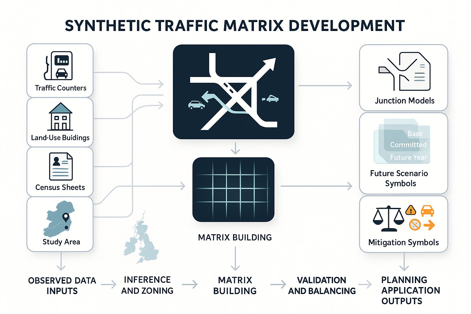
When a planning application depends on credible transport evidence, one weak input can unravel the whole assessment: the traffic demand matrix. In practice, we’re not always handed pristine origin–destination survey data for every movement through a study area. More often, we have partial counts, turning movements, local knowledge, land-use context, and a network that still needs to be tested properly. That’s where synthetic traffic matrix development becomes essential.
For architects, planners, developers, councils, and legal teams, this matters because junction modelling is only as reliable as the demand fed into it. If the matrix is unrealistic, the model can look precise while telling the wrong story. And that’s usually where objections, delay, or costly rework begin.
In our work on planning-led transport assessments, we use synthetic matrices to bridge the gap between observed traffic data and the practical need to assess base, committed, and future-year scenarios. Done well, they provide a defensible, transparent representation of how trips are likely to move across the network. Done badly, they create obvious inconsistencies that reviewers will spot quickly.
This guide explains what a synthetic traffic matrix is, how it is built, where the evidence comes from, and how to present it clearly in a planning report. The aim is simple: help teams understand what good looks like, and why a robust matrix can make the difference between a smooth planning process and a very long one.
What A Synthetic Traffic Matrix Is And When It Is Used
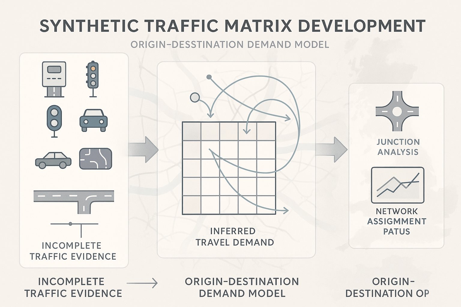
A synthetic traffic matrix is an estimated origin–destination representation of traffic demand created where full direct O-D survey data does not exist, is incomplete, or would be disproportionate to collect. In simple terms, it tells us how many vehicles are likely to travel from each origin zone to each destination zone within a modelled network.
In planning work, this matrix sits behind much of the testing. It provides the demand layer used in transport assessment, junction modelling, network assignment, and future-year forecasting. Without it, we may know that vehicles passed a count point, but we do not properly understand how those vehicles connect across the wider system.
Synthetic traffic matrix development is most commonly used when we have a sensible package of observed data, link counts, turning counts, classified surveys, ATCs, and local network information, but not a complete picture of trip origins and destinations. That is normal on planning projects. Full roadside interviews, ANPR-based O-D capture, or mobile data may be unavailable, unnecessary, or too costly for the scale of the application.
So we infer. We assemble the best available evidence, establish plausible movement patterns, and create a matrix that can be assigned through the network and checked against observed flows. The key point is that “synthetic” does not mean speculative. It should mean evidence-led, transparent, and proportionate to the planning question being asked.
Why Planning Applications Need A Robust Matrix
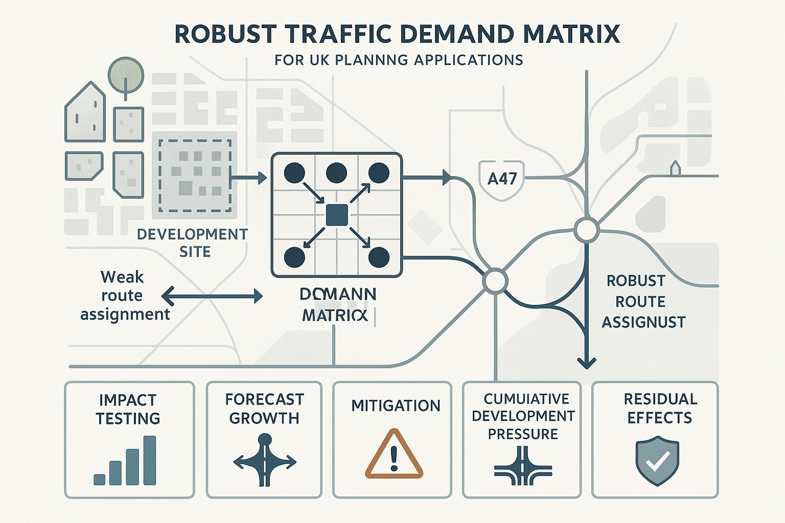
Planning applications need a robust matrix because impact assessment is not just about counting traffic at a site access. We need to understand where traffic comes from, where it goes, which routes it uses, and how those movements interact with nearby junctions under existing and future conditions.
A weak matrix can distort all of that. It may overstate pressure on one arm of a junction, understate demand at another, or assign trips along routes no local driver would reasonably choose. On paper, the model still runs. But the conclusions become fragile, and that creates risk for applicants, consultants, and decision-makers alike.
For local planning authorities, a robust matrix gives confidence that the submitted transport assessment is based on realistic demand. For developers and design teams, it reduces the chance of challenge late in the process. For lawyers and planning advisers, it provides a clearer evidence trail if technical assumptions are scrutinised.
This is especially important in 2026, when planning decisions are often taken against a backdrop of constrained networks, cumulative development pressure, and closer review of assumptions around mode share and trip generation. A sound synthetic matrix helps us test not only the base case, but also committed development, forecast growth, mitigation, and residual effects.
In short: if the matrix is credible, the modelling discussion becomes more productive. If it is not, everything downstream becomes harder.
The Main Data Sources Used To Build A Synthetic Matrix
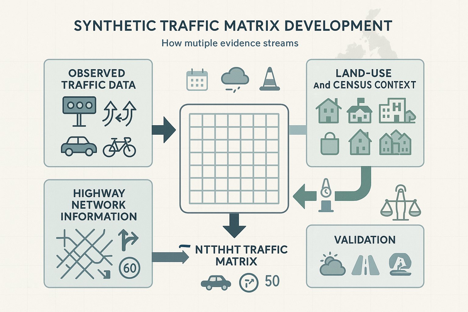
A synthetic matrix should never be built from one data source alone. The most reliable results come from layering observed surveys with land-use and network context, then checking that the emerging demand pattern makes sense both numerically and geographically.
In most planning-led studies, we start with observed traffic data because it anchors the matrix to real-world conditions. We then use broader contextual datasets to infer the missing connections between count sites, define zones, and estimate likely trip distribution patterns.
The quality of the final matrix depends heavily on whether those datasets are compatible. Count dates, school term conditions, temporary roadworks, weather disruption, and seasonal distortions all matter more than people sometimes assume. A “good” count can still be the wrong count if it reflects an abnormal network.
The best approach is usually pragmatic rather than elaborate: use enough evidence to explain traffic behaviour credibly, and document why each source was chosen.
Traffic Counts, Turning Counts, And Classified Surveys
Traffic counts are the backbone of most synthetic traffic matrix development. Automatic traffic counts help us understand hourly variation, daily profiles, and directional flow. Manual classified counts give richer detail at junctions, showing how traffic actually turns between arms during the critical peaks. That turning information is often what allows us to trace likely through-movements between adjacent nodes.
Classified data also matters because not all vehicles behave the same way. Cars, LGVs, and HGVs can have different routing patterns, operating periods, and sensitivity to constraints. Where a development has a freight element, or where local restrictions affect larger vehicles, class-specific treatment is often essential.
The practical challenge is that counts rarely line up perfectly. One junction may show more outbound flow than the next junction shows inbound. That is normal. We reconcile those differences through matrix estimation and balancing rather than assuming the surveys are unusable.
Land Use, Census, And Highway Network Information
Observed counts tell us what happened at survey points. Land-use, census, and highway network information help explain why it happened, and where trips are likely to start or end.
Land-use context is particularly useful when defining zones and testing plausibility. Retail parks, schools, employment areas, housing estates, hospitals, and town centres generate very different movement patterns. If the matrix implies large flows to or from places with no obvious trip attraction, that is usually a warning sign.
Census journey-to-work data can still offer useful directional insight, especially for broader commuting patterns, even though it should not be treated as a direct traffic assignment dataset. We use it carefully, as one input among several. Highway network information is equally important: route hierarchy, one-way systems, banned turns, speed environment, signal control, and known rat-runs all influence likely path choice.
When these datasets are combined properly, they stop the matrix becoming a purely mathematical exercise. They keep it grounded in how the area actually functions.
How Existing Demand Is Estimated Across The Network
Estimating existing demand across a network usually begins with observed flows at key screenlines and junctions, then works outward to identify how those flows must connect. We are effectively solving a puzzle with some pieces missing: we know what entered and left parts of the network, and we need to infer the internal movement pattern that best explains those observations.
A common method is to trace plausible movement paths between count locations using the network structure and turning data. If one junction records strong northbound through-demand and the next junction downstream shows corresponding arrivals, we can start building a consistent picture of existing movement. Where the numbers do not reconcile neatly, we assess whether the gap is likely to arise from local access activity, survey variance, uncontrolled side roads, or route alternatives.
Zoning matters here. If zones are too coarse, the matrix hides important local detail. If they are too fine, it becomes unstable and overly sensitive to weak assumptions. Good zoning reflects the geography of trip-making and the level of modelling required for the planning issue.
At this stage, professional judgement matters as much as arithmetic. We want the matrix to fit counts, yes, but we also want it to reflect realistic travel behaviour. An exact fit built on implausible routing is not a robust base model.
How Origin-Destination Patterns Are Inferred Without Direct O-D Surveys
Without direct O-D surveys, we infer origin-destination patterns from a mix of observed traffic behaviour, land-use relationships, route choice logic, and trip-cost assumptions. That sounds technical, but the principle is straightforward: drivers do not move randomly, and the network leaves clues.
One approach is synthetic distribution based on known attractions and productions across zones. Another is a gravity-style method, where trips are more likely between places with stronger trip-making potential and lower perceived separation. “Separation” might reflect distance, time, congestion, route quality, or barriers such as river crossings and one-way systems.
Turning counts are often the bridge between local observation and wider inference. They show how traffic entering a node splits by direction, which can then inform the likely continuation of trips through the surrounding network. If several adjacent junctions tell a consistent directional story, we can derive a plausible O-D structure even without number-plate matching or roadside interviews.
Of course, this is where synthetic traffic matrix development can either look thoughtful or look shaky. Unrealistic long-distance local movements, excessive use of minor roads, or improbable cross-town routing patterns are red flags. We hence test the inferred patterns against local knowledge and observed congestion. If the matrix says one thing but everyone familiar with the area knows another, we go back and fix it.
Methods For Balancing And Validating The Matrix
Once an initial matrix has been built, it needs to be balanced and validated. In practice, that means adjusting demand iteratively so that assigned flows align reasonably with observed counts while preserving realistic movement structure.
Balancing typically seeks consistency between row and column totals and target flows at key points in the network. Matrix estimation tools can do this mathematically, but the process still needs supervision. If an algorithm improves count fit by producing odd routing patterns or unstable trip patterns, the answer is not to accept it blindly because the statistics look tidy.
Validation is about demonstrating that the matrix performs acceptably against observed conditions. Depending on the study, that may involve comparing modelled and surveyed link flows, turning movements, and journey patterns across the network. A commonly used sense-check is whether differences are broadly within around 5% at critical locations, though the acceptable threshold depends on model type, data quality, and authority expectations.
We also look for consistency rather than isolated “wins”. A matrix that fits one junction beautifully but misses the surrounding area is not validated in any meaningful planning sense. The objective is a coherent, defensible representation of demand. At ML Traffic, that usually means prioritising transparency: showing what was adjusted, why it was adjusted, and where limitations remain.
Factoring Development Traffic Into The Base And Future-Year Matrices
Once the base matrix is accepted, development traffic can be added for testing. This step sounds simple, but it is often where strategic mistakes creep in.
First, we establish the site-generated trips using the agreed trip generation and distribution assumptions. Those trips then need to be loaded onto the correct base-year matrix or scenario matrix, not simply dropped into a model in isolation. The surrounding network is already carrying demand: development traffic changes how that demand interacts at key junctions.
For future-year assessment, the process is usually layered. We start with a base matrix, apply background growth where appropriate, account for committed developments, and then add the proposed development traffic. Depending on the modelling framework, internalisation, pass-by trips, reassignment, and mode share assumptions may also need to be reflected.
The important point is consistency. If the development trip distribution assumes one pattern but the base synthetic matrix implies a conflicting route logic, the forecast becomes harder to defend. The same applies where committed schemes alter route choice but the matrix has not been updated to reflect those changes.
A good future-year matrix is not just “bigger” than the base matrix. It is structurally credible. And in planning terms, that is what allows us to test mitigation and residual impact with confidence.
Peak Period Selection, Vehicle Classes, And Time-Slice Decisions
Peak period selection can make or break the usefulness of a matrix. Planning assessments usually focus on network conditions when pressure is highest, but the “peak” is not always the standard weekday commuter hour. For schools, retail, logistics, leisure, or mixed-use sites, the critical period may be different from the default assumptions.
That is why we start with evidence. ATC profiles, local count data, site context, and authority expectations should guide the selection of AM, PM, inter-peak, Saturday, or bespoke assessment periods. Choosing the wrong peak can lead to an apparently compliant assessment that misses the actual stress point.
Vehicle classes also deserve care. A single all-vehicle matrix may be enough for some schemes, but many applications benefit from separating cars, light goods vehicles, and heavy goods vehicles. Different classes have different growth patterns, routing constraints, and operational implications, especially at tight junctions or on roads with environmental sensitivities.
Then there is the question of time slices. For LINSIG, ARCADY, PICADY, or microsimulation work, 15-minute demand profiles may be necessary even where hourly matrices exist. If the peak quarter-hour is materially sharper than the average hour, smoothing demand can understate queueing and delay. So we do not just ask, “What data do we have?” We ask, “What temporal resolution does the decision actually require?”
Common Errors That Undermine Matrix Credibility
Most weak matrices do not fail because of one dramatic mistake. They fail because several smaller issues combine into something reviewers no longer trust.
One common problem is inconsistent survey data: counts taken on different dates, in different months, or under abnormal conditions, then treated as though they describe one stable network. Another is poor zoning, where the model is either so aggregated that it conceals key local movements or so fragmented that it invents precision without evidence.
Unrealistic routing is another frequent issue. If the matrix sends substantial traffic along minor residential streets, banned turns, or obviously unattractive routes, credibility drops very quickly. The same happens when gaps between survey sites are ignored rather than explained. Missing side-road demand, local access traffic, and short internal trips can all distort balancing if left unresolved.
There is also a reporting problem. Some matrices may be technically salvageable, but the supporting note does not explain assumptions clearly enough for anyone else to follow. That is risky in planning.
In our experience, the best safeguard is simple: challenge the matrix as if you were reviewing it for the local authority. Does it fit counts? Does it reflect the network? Does it make everyday sense? If not, it probably needs more work.
How Synthetic Traffic Matrices Support Junction Modelling And Transport Assessment
A synthetic matrix is not an end in itself. Its value lies in what it enables us to test.
For junction modelling, the matrix provides the demand input that drives operational assessment. Whether we are using priority, roundabout, signal, or wider network models, we need a realistic pattern of traffic entering, passing through, and leaving the system. Turning counts alone may describe one surveyed moment at one junction: a matrix links that junction to the wider movement context.
That matters particularly where developments influence several nodes rather than one access point. A robust synthetic matrix allows traffic to be assigned across the study area so we can examine queueing, reserve capacity, delay, and interaction effects in a more coherent way. It also supports comparison between scenarios: base, future year, with development, and with mitigation.
For the transport assessment itself, the matrix underpins the narrative around impact. It helps show why particular junctions were tested, how distribution assumptions were derived, and whether observed and forecast patterns are consistent with local conditions. This is often the difference between a report that merely presents outputs and one that genuinely explains them.
In planning terms, that clarity is useful for everyone involved, applicants, officers, members, and sometimes inspectors. A good matrix turns modelling from a black box into evidence.
Presenting Assumptions, Limitations, And Results Clearly In Planning Reports
Even a well-built matrix can become vulnerable if it is presented badly. Planning reports should explain, plainly and in sequence, what data was used, what the study area covers, how zones were defined, which time periods were assessed, how vehicle classes were treated, and what balancing or estimation process was applied.
We should also be honest about limitations. If direct O-D survey data was not available, say so. If one count location was affected by an abnormal event and required adjustment, document it. If the matrix fits most locations well but remains weaker at a peripheral arm with limited influence on the development impact, explain that too. Reviewers are generally more comfortable with a transparent limitation than with an unexplained inconsistency.
Tables and figures help, but only if they are selective and readable. A concise matrix methodology section, flow comparison tables, turning diagrams, and a short note on assumptions usually do more good than pages of opaque appendices dropped in without comment.
And the tone matters. We should not oversell a synthetic matrix as though it were direct observation. It is an informed estimate, validated against evidence and suited to the planning purpose. Presented that way, it becomes far easier for decision-makers to rely on.
In the end, clear reporting is not decoration. It is part of the technical case, and often the part people remember when the application is reviewed.
Frequently Asked Questions about Synthetic Traffic Matrix Development
What is a synthetic traffic matrix and when is it used in transport assessment?
A synthetic traffic matrix is an estimated origin–destination representation of traffic demand created when full direct O-D survey data is unavailable or incomplete. It is used to distribute trips across a network for transport assessment, junction modelling, and future-year forecasting in planning projects.
Why is a robust synthetic traffic matrix essential for planning applications?
A robust synthetic traffic matrix provides realistic traffic demand patterns necessary to test junction performance and network impacts under existing and future conditions. It ensures credible modelling outputs, reducing the risk of objections, delays, or costly rework in the planning process.
Which main data sources are used to build a synthetic traffic matrix?
Key inputs include observed traffic counts, manual classified surveys, automatic traffic counts, turning movement data, land-use information, census journey-to-work data, and highway network characteristics. Combining these ensures the matrix is evidence-led and reflects local travel behaviour.
How are origin–destination traffic patterns inferred without direct O-D surveys?
Without direct surveys, O-D patterns are inferred by analysing observed turning movements, land-use relationships, route choice logic, and trip-cost assumptions using synthetic distribution or gravity-based methods to estimate likely flows between zones across the network.
How is a synthetic traffic matrix validated and balanced for accuracy?
Matrices are balanced iteratively so that row and column totals match observed traffic counts. Validation involves checking modelled flows against surveyed link and turning counts, aiming for differences generally within about 5% at key locations, ensuring movement patterns remain realistic and consistent.
How does synthetic traffic matrix development support junction modelling and future-year transport assessment?
Synthetic traffic matrices provide the demand input driving junction and network models, enabling analysis of traffic flow, queueing, and delay under base, committed development, and future scenarios. This supports confident testing of mitigation measures and impact forecasting in transport assessments.